Introduction

This application is a web base tool that allows the users to explore the different hierarchies of data that combine to form an image (render) using Path Tracing techniques. The user can further identify problematic sample, path lengths, or objects and remove them or alter them to fit their need by sending representative of problematic data to the server which in turn will process the statistical data and return a new render. Furthermore the user is able to detect and fix problematic pixels with a high-level approach using automatic "firefly" detection and removal tools.

Furthermore the user is able to detect and fix problematic pixels with a high-level approach using automatic "firefly" detection and removal tools.

Tools

The following tools and technologies have been used extensively throughout this project:

• D3.js
• D3 is used to construct and manipulate the different windows, and dynamically display relevant information.
• jQuery
• jQuery is used extensively for easy access of and manipulation of DOM elements and UI elements.
• HTML5 Canvas Element
• Canvas elements are used throughout the project for modification and accessing pixel data using selectors or through algorithmic procedures.
• Cropper.js
• Cropper.js is provides easy to use API for cropping and manipulating images.
• Bootstrap
• Bootstrap is utilized to provide a responsive and uniform display.

Features

This visualization project provides a wide range of image and data inspection. Furthermore our approach in data allows other developers who work on open-source rendering engines to be able to easily integrate out front-end with their backend and provide a solution to other enthusiasts.

Each tool has self-explanatory description, and to reduce confusion every element is document as much as possible to guide the user through the data, and process.

Background and Motivation

Bidirectional path tracing is a physically-based rendering technique. In many cases it is capable of producing a rendered image that is practically indistinguishable from a photograph. The rendering program attempts to simulate the physical properties of all elements of a scene, including lights, geometric objects, materials, and cameras. Path tracing is a Monte-Carlo integration technique that generates paths using probability distributions.

Regular (unidirectional) path tracing starts by choosing a random position on the film plane and then randomly choosing a position on the camera aperture. These two choices will create a ray that shoots from the camera into the scene. Every time the ray intersects a surface, the material properties of the surface are used to choose a new direction to travel in. The ray continues to bounce around the scene until one of three conditions is met. The ray may hit a light creating a complete path, at which point the ray’s path is terminated. Alternatively, the ray may have bounced so many times that we choose to terminate it. Lastly, the scene might be open and the ray may have gone off into outer space (a non-hit). Every surface interaction, including the camera, is called a vertex. A complete path starts at the camera and ends at a light, and every vertex contains information needed to calculate the final color contribution for that path.

Project Objectives

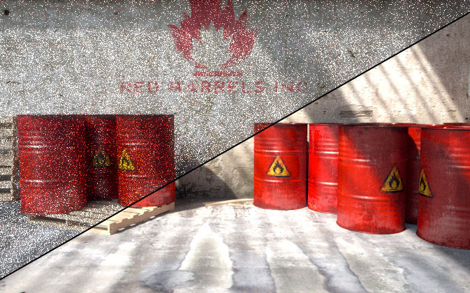
The main purpose of this visualization project is to provide an overview of the rendering process and make it easy to explore how the image was created and possibly identify problematic pixel samples. This allows the artist/developer to understand and determine the components of the scene that result in low-probability paths that can lead to noise in the final image. Such low-probability paths can result in outlier pixels, informally referred to as fireflies, that do not fit in terms of color with their neighboring pixels due to intense brightness. Through visualizing path statistics and probabilities, one could easily trace the source of the error and proceed with modifying the image to eliminate the outlier pixel samples, or conversely changing the scene to make rendering easier.

There is one question that is very important to answer, which samples cause a pixel to be a great deal brighter than it should be. These outlier pixels or “fireflies” are a common nuisance in rendering, and can come from many difference sources. These bad samples are not incorrect, strictly speaking, but would require a very high number of samples in order to average to the expected (correct) color value. That is because these are usually very low probability samples. We possibly need an unreasonably large number of samples to get a substantial set of these rare samples. In order to produce a nice image in a reasonable amount of time, it is often more pragmatic to simply remove these samples from the image.

Data

The actual data is generated as a matter of course during the rendering process. Normally this data is generated iteratively, processed to get a final color value, and then discarded in order to minimize memory usage. Since there will be a large amount of data, I have decided to store everything in a database. The database may need to be optimized for queries, since fetching data may cause a bottleneck. Our rendering program is smallpt, written in C++ by Kevin Beason. It features Global illumination via unbiased Monte Carlo path tracing and Specular, Diffuse, and Glass BRDFs. The data was stored as a series of JSON files for each pixel and samples.

Data Representation

Data is broken up into a hierarchy of four levels. At the root we the actual image which contains a series of pixels, each containing four values for Red, Blue, Green, and Alpha channels. This information is simply inferred from the received image.

Next, for each pixel, there exists a collection of sample that contribute to the final color value of the pixel. We use the following scheme for representing sample collections.

                        
{"samples": [
	{"uid": "S-X-Y-0", "final_contribution": 0.00000, "red": 0.00000, "green": 0.00000, "blue": 0.00000},
	{"uid": "S-X-Y-1", "final_contribution": 0.00000, "red": 0.00000, "green": 0.00000, "blue": 0.00000},
	{"uid": "S-X-Y-2", "final_contribution": 0.00000, "red": 0.00000, "green": 0.00000, "blue": 0.00000},
	{"uid": "S-X-Y-3", "final_contribution": 0.00000, "red": 0.00000, "green": 0.00000, "blue": 0.00000},
	{"uid": "S-X-Y-4", "final_contribution": 0.00000, "red": 0.00000, "green": 0.00000, "blue": 0.00000},
	{"uid": "S-X-Y-5", "final_contribution": 0.00000, "red": 0.00000, "green": 0.00000, "blue": 0.00000},
	{"uid": "S-X-Y-6", "final_contribution": 0.00000, "red": 0.00000, "green": 0.00000, "blue": 0.00000},
]}
                    
                    

The S-X-Y-N ID of each sample represents the pixel it belongs to using the X and Y values which respectively correspond to the row and column of the pixel in the image. The last integer N is the unique index of the sample for that pixel. S is simply a prefix that identifies this object as a Sample.

Each sample consists of a unique ID which was explained above, as well as a final_contribution value which signifies the importance of the sample in the context of the parent pixel, as well as RGB values. A sample is in turn a product of a number of paths. And yet each path itself is formed from a ray bouncing from different objects. We represents the paths and vertices collections as follows.

                        
{"paths": [
	{"uid": "P-X-Y-S-0", "weight": 0.25, "red": 0, "green": 0, "blue": 0,
		"veredtices": [
			{"oblueject_id": 3, "red": 0.00000, "green": 0.00000, "blue": 0.00000},
			{"oblueject_id": 5, "red": 0.00000, "green": 0.00000, "blue": 0.00000},
			{"oblueject_id": 3, "red": 0.00000, "green": 0.00000, "blue": 0.00000},
			{"oblueject_id": 5, "red": 0.00000, "green": 0.00000, "blue": 0.00000},
			{"oblueject_id": 4, "red": 0.00000, "green": 0.00000, "blue": 0.00000},
			{"oblueject_id": 0, "red": 0.00000, "green": 0.00000, "blue": 0.00000},
			{"oblueject_id": 4, "red": 0.00000, "green": 0.00000, "blue": 0.00000}
		]
	},
	{"uid": "P-X-Y-S-1", "weight": 0.25, "red": 0, "green": 0, "blue": 0,
		"veredtices": [
			{"oblueject_id": 3, "red": 0.00000, "green": 0.00000, "blue": 0.00000},
			{"oblueject_id": 0, "red": 0.00000, "green": 0.00000, "blue": 0.00000},
			{"oblueject_id": 3, "red": 0.00000, "green": 0.00000, "blue": 0.00000},
			{"oblueject_id": 0, "red": 0.00000, "green": 0.00000, "blue": 0.00000},
			{"oblueject_id": 4, "red": 0.00000, "green": 0.00000, "blue": 0.00000},
			{"oblueject_id": 5, "red": 0.00000, "green": 0.00000, "blue": 0.00000},
			{"oblueject_id": 4, "red": 0.00000, "green": 0.00000, "blue": 0.00000},
			{"oblueject_id": 5, "red": 0.00000, "green": 0.00000, "blue": 0.00000}
		]
	}
]}
                    
                    

Similarly P-X-Y-S-N ID of each path represents its unique index N in the sample S that it belongs to, as well as the pixel the sample belongs to using the X and Y values which respectively correspond to the row and column of the pixel in the image. P is simply a prefix that identifies this object as a Path.

As displayed, a path in our representation consists a number of vertices, each having their own value of RGB. The path itself also is represented using RGB and in this case a uniform weight.